High Level description of the EMIR Data Reduction Pipeline
- author:
Nicolás Cardiel, Sergio Pascual
- revision:
1
- date:
2008-02-09
Warning
The following content is an overall description of the relevant processes initially planned to be incorporated into PyEmir. Note, however, that the final implementation of the data reduction pipeline may differ with respect to these initial guidelines.
Introduction
The information here contained follows the contents of the EMIR Observing Strategies document.
The reason for a data reduction
The data reduction process, aimed to minimize the impact of data acquisition imperfections on the measurement of data properties with a scientific meaning for the astronomer, is typically performed by means of arithmetical manipulations of data and calibration frames.
The imperfections are usually produced by non-idealities of image the sensors: temporal noise, fixed pattern noise, dark current, and spatial sampling, among others. Although appropriate observational strategies can greatly help in reducing the sources of data biases, the unavoidable limited observation time that can be spent in each target determines the maximum signal-to-noise ratio in practice achievable.
Sources of errors
- Common sources of noise in image sensors are separated into two categories:
Random noise: This type of noise is temporally random (it is not constant from frame to frame). Examples of this kind of noise are the followings:
Shot noise: It is due to the discrete nature of electrons. Two main phenomena contribute to this source of error: the random arrival of photo-electrons to the detector (shot noise of the incoming radiation), and the thermal generation of electrons (shot noise of the dark current). In both cases, the noise statistical distributions are well described by a Poisson distribution.
Readout noise: Also known as floor noise, it gives an indication of the minimum resolvable signal (when dark current is not the limiting factor), and accounts for the amplifier noise, the reset noise, and the analog-to-digital converter noise.
Pattern noise: it is usually similar from frame to frame (i.e. it is stable in larger timescales), and cannot be reduced by frame averaging. Pattern noise is also typically divided into two subtypes:
Fixed Pattern Noise (FPN):This is the component of pattern noise measured in absence of illumination. It is possible to compensate for FPN by storing the signal generated under zero illumination and subtracting it from subsequent signals when required.
Photo-Response Non-Uniformity (PRNU): It is the component of pattern noise that depends on the illumination (e.g. gain non-uniformity). A first approximation is to assume that its contribution is a (small) fraction,
 , of the number of photo-electrons,
  .
Under this hypothesis, and considering in addition only the shot
noise due to photo-electrons, the resulting variance of the combination
of both sources of noise would be expressed as
.
Under this hypothesis, and considering in addition only the shot
noise due to photo-electrons, the resulting variance of the combination
of both sources of noise would be expressed as
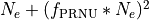 Thus, the worst case is obtained when approaches
the pixel full-well capacity.
Thus, the worst case is obtained when approaches
the pixel full-well capacity.
It is important to note that the correction of data biases, like the FPN, also constitutes, by itself, a source of random error, since they are performed with the help of a limited number of calibration images. In the ideal case, the number of such images should be large enough to guarantee that these new error contributors are negligible in comparison with the original sources of random error.
Basic observing modes and strategies
EMIR is offering two main observing modes:
imaging: FOV of 6.67 x 6.67 arcmin, with a plate scale of 0.2 arcsec/pixel. Imaging can be done through NIR broad-band filters Z, J, H, K, Ks, and a dataset of narrow-band filters (TBC).
multi-object spectroscopy: multi-slit mask with a FOV of 6.67 x 4 arcmin. Long-slit spectroscopy can be performed by placing the slitlets in adjacent positions.
We are assuming that a particular observation is performed by obtaining a set of images, each of which is acquired at different positions referred as offsets from the base pointing. In this sense, and following the notation used in EMIR Observing Strategies, several situations are considered:
Telescope
Chopping (TBD if this option will be available): achieved by moving the GTC secondary mirror. It provides a 1D move of the order of 1 arcmin. The purpose is to isolate the source flux from the sky background flux by first measuring the total (Source+Background) flux and then subtracting the signal from the Background only.
DTU Offseting: the Detector Translation Unit allows 3D movements of less than 5 arcsec. The purpose is the same as in the chopping case, when the target is point-like. It might also be used to defocus the target for photometry or other astronomical uses.
Dither: it is carried out by pointing to a number of pre-determined sky positions, with separations of the order of 25 arcsec, using the GTC primary or secondary mirrors, or the EMIR DTU, or the Telescope. The purpose of this observational strategy is to avoid saturating the detector, to allow the removal of cosmetic defects, and to help in the creation of a sky frame.
Nodding: pointing the Telescope alternatively between two or more adjacent positions on a 1D line, employing low frequency shifts and typical distances of the order of slitlet-lengths (it plays the same role as chopping in imaging).
Jitter: in this case the source falls randomly around a position in a known distribution, with shifts typically below 10 arcsec, to avoid cosmetic defects.
Imaging Mode
In near-infrared imaging it is important to take into account that the variations observed in the sky flux in a given image are due to real spatial variations of the sky brightness along the field of view, the thermal background, and intrinsic flatfield variations.
The master flatfield can be computed from the same science frames (for small targets) or from adjacent sky frames. This option, however, is not the best one, since the sky brightness is basically produced by a finite subset of bright emission lines, which SED is quite different from a continuous source. For this reason, most of the times the preferred master flatfield should be computed from twilight flats. On the other hand, systematic effects are probably more likely in this second approach. Probably it will be required to test both alternatives. The description that follows describes the method employed when computing the master flatfield from the same set of night images, at is based on the details given in SCAM reduction document, corresponding to the reduction of images obtained with NIRSPEC at Keck II.
A typical reduction scheme for imaging can be the following:
Data modelling (if appropriate/possible) and variance frame creation from first principles: all the frames
Correction for non-linearity: all the frames
Data:
Variances:
Dark correction: all the frames
Data:
Variances:
Master flat and object mask creation: a loop starts

![\sigma^2_{\mathrm{linear}}(x,y)=[\sigma_{\mathrm{model}}(x,y) \mathrm{Pol}_{\mathrm{linearity}}]^2 + [I_{\mathrm{observed}}(x,y) \mathrm{ErrorPol}_{\mathrm{linearity}}]^2](../_images/math/851f2f83772f40af1c1b60dabc8dfa8282fad84a.png)

![\sigma^2_{dark}(x,y)=[\sigma_{linear}(x,y)]^2 + [ErrorMasterDark(x,y)]^2](../_images/math/fd56522bdc976dc69ce9e2b612ab03afb23009d0.png)
First iteration: computing the object mask, refining the telescope offsets, QC to the frames.
No object mask is used (it is going to be computed).
All the dark-corrected science frames are used.
No variances computation.
BPM is used.
Flat computation (1st order):
Combination using the median (alternatively, using the mean).
No offsets taken into account.
Normalization to the mean.
Flat correction (1st order):
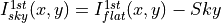
Sky correction (1st order):
Sky is computed and subtracted in each array channel (mode of all the pixels in the channel), in order to avoid time-dependent variations of the channel amplifiers.
BPM is used for the above sky level determination.
Science image (1st order):
Combination using the median.
Taking telescope offsets into account.
Extinction correction is performed to each frame before combination:
, being
the airmass.
Rejection of bad pixels during the combination (alternatively, asigma-clipping algorithm).
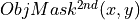
Object Mask (1st order):
High DETECT_THRESH (for detecting only the brightest objects).
Saturation limit must be carefully set (detected objects must not be saturared).
Offsets refinement:
Objects are also found in the sky-corrected frames:
All the objects detected in the combined science image are also identified in each sky-corrected frame. For doing that, the position of each source from the combined image is converted into positions in the reference system of each frame
. The telescope offsets are used for a first estimation of the source position in the frame. A TBD cross-correlation algorithm finds the correct source position into a window of size S around the estimated position. The new improved offsets are computed for each source in each frame.
The differences between the improved offsets (OFFX, OFFY) and the telescope (nominal) offsets (OFFXtel, OFFYtel) are computed for each object in each frame.
The differences between both sets of offsets are plotted for all the objects vs. Object Number, ordered by brightness.
The mean values of these differences (weighting with object brightness) are computed, making an approximation to integer values. These values represent the average displacement of the true offsets of the frame relative to the nominal telescope offsets.
If the estimated refined offsets are very different from the nominal values, the
image is computed again, using the refined offset values. A llop starts from step d) to f), until the offsets corrections are less than a TBD threshold value for the corresponding frame.
Quality Control for the science frames:
The brightest objects detected in the
are selected (N~5 objects). They must appear in more than two frames.
The FLUX_AUTO and the FWHM of each selected object are computed in each frame.
The
and FWHM are plotted vs. frame number.
The median values of
A sigma-clipping algorithm will select those frames with more than N/2 objects (TBD) lying +/- 1 sigma above/below the median value of
All those frames with FWHM lying n times sigma above their median value or m times sigma below it are also flagged as non-adequate. Notice that m and n must be different (FWHM values better than the median must be allowed).
The non-adequate frames are not used for generating the final science frame. They will be avoided in the rest of the reduction.
A QC flag will be assigned to the final science image, depending on the number of frames finally used in the combination. E.g, QC_GOOD if between 90-100% of the original set of frames are adequate, QC_FAIR between 70-90%, QC_BAD below 70% (the precise numbers TBD).
![Flat^{1st}(x,y)=\mathrm{Comb}[I_{dark}(x,y)]/\mathrm{Norm}](../_images/math/1d5c22c878fa53e1a13701cdb427d48abe3e643c.png)

![Science^{1st}(x,y)=Comb[I_{sky}^{1st}(x,y)]](../_images/math/451c57f2167f07e7c74b6c1cc043f139e5f21521.png)
![SExtractor[Science^{1st}(x,y)] -> Obj_Mask^1st(x,y)](../_images/math/7e0353a8ff814bd463557e8f673ab476abeceac5.png)
![SExtractor[I_{sky}^{1st}(x,y)]](../_images/math/add6047bf3c30021d227e701fd4e955030d5e23f.png)
Second iteration
- is used for computing the flatfield and the sky.
Only those dark-corrected science frames that correspond to adequate frames are used.
No variances computation.
BPM is also used.
Flat computation (2nd order):
Combination using the median (alternatively, using the mean).
The first order object mask is used in the combination.
No offsets taken into account in the combination, although they are used for translating positions in the object mask to positions in each individual frame.
Normalization to the mean.
Flat correction (2nd order):
Sky correction (2nd order):
is computed as the average of m (~ 6, TBD)
frames, near in time to the considered frame, taking into account the first order object mask and the BPM.
An array storing the number of values used for computing the sky in each pixel is generated (weights array).
If no values are adequate for computing the sky in a certain pixel, a zero is stored at the corresponding position in the weights array. The sky value at these pixels is obtained through interpolation with the neighbouring pixels.
Science image (2nd order):
Combination using the median.
Taking the refined telescope offsets into account.
Extinction correction is performed to each frame before combination:
Rejection of bad pixels during the combination (alternatively, asigma-clipping algorithm).
Object Mask (2nd order):
Lower DETECT_THRESH.
Saturation limit must be carefully set.
![Flat^{2nd}(x,y)=Comb[I_{dark}(x,y)]/Norm](../_images/math/61920a92281dd1a8cb3a4e858933eccbf6ff6938.png)


![Science^{2nd}(x,y)=Comb[I_{sky}^{2nd}(x,y)]](../_images/math/c94b2b18e1f5dbc614f2a81588d49c8a85c65ad1.png)
![SExtractor[Science^{2nd}(x,y)] -> ObjMask^{2nd}(x,y)](../_images/math/3b3e6d9955ac9ef02e7e1fb448b2ebebf41e9d4c.png)
Third iteration
 is used in the combinations.
Only those dark-corrected science frames that correspond to adequate frames are used.
Variance frames are computed.
BPM is also used.
Additional iterations: stop the loop when a suitable criterium applies (TBD).
Multi-Object Spectroscopy Mode
In the case of EMIR, the reduction of the Multi-Object Spectroscopy observations will be in practice carried out by extracting the individual aligned slits (not necessarily single slits), and reducing them as if they were traditional long-slit observations in the near infrared.
Basic steps must include:
Data modelling (if appropriate/possible) and variance frame creation from first principles: all the frames
Correction for non-linearity: all the frames
Data:
Variances:
Dark correction: all the frames
Data:
Variances:
Flatfielding: distinguish between high frequency (pixel-to-pixel) and low-frequency (overall response and slit illumination) corrections. Lamp flats are adequate for the former and twilight flats for the second. Follow section
Detection and extraction of slits: apply Border_Detection algorithm, from own frames or from flatfields.
Cleaning
Single spectroscopic image: sigma-clipping algorithm removing local background in pre-defined direction(s).
Multiple spectroscopic images: sigma-clipping from comparison between frames.
Wavelength calibration and C-distortion correction of each slit. Double-check with available sky lines.
Sky-subtraction (number of sources/slit will be allowed to be > 1?).
Subtraction using sky signal at the borders of the same slit.
Subtraction using sky signal from other(s) slit(s), not necessarily adjacent.
Spectrophotometric calibration of each slit, using the extinction correction curve and the master spectrophotometric calibration curve.
Spectra extraction: define optimal, average, peak, FWHM.

![\sigma^2_{linear}(x,y)=[\sigma_{model}(x,y) Pol_{linearity}]^2 + [I_{observed}(x,y) ErrorPol_{linearity}]^2](../_images/math/e0ceb07150154469a43b299dcf33f74c2c0d721e.png)
